Profiling

Let’s say you have a more complicated piece of code that you are trying to optimise. Many functions are very complex and call other nested functions, and it would be tedious to try and benchmark each individual line of code in this algorithm, and maybe that’s not even possible, since you are using some else’s code and cannot edit their source code directly. What can you do?

This is where profiling comes into play. Profiling can allow you to diagnose poor performing parts of your code base. It does this by running your program as normal and inspecting which parts of the code get called and for how long. There are many implementations for achieving this, but we will only talk about statistical profilers.

A statistical profiler works by frequently asking the operating system which part of the program is running at any different time. This is used to build up a picture of which part of the code is being executed for the longest amount of time during the lifetime of the program. This method can be very good as it allows the code to run at close to full speed while the profile is being collected. The downside is that this method is often prone to numerical errors and mistakes and is often unsuitable for some tasks. This is the main way that Julia allows for profiling in the language. The built-in library Profile.jl contains tools for profiling your code and the external package PProf.jl contains tools to let you visualise the profile results. An example of using these tools to diagnose memory allocations is provided in the next section, but applies to testing speed by removing the Allocs submodule from each of the commands.

A profiler is quite good at identifying the relatively slow parts of your code. If you have a block of code that takes 95% of the execution time, it is worth focusing on that block instead of any code in the other 5%. This is important to recognise, since profiling can be very informative, often times independent of the hardware the program is being run on. This approach will be used frequently to identify slow running parts of your code. Often times, most programs have a hot loop, which repeatedly executes code many times. It is often work identifying this hot loop and optimising the inner function before anything else.

Example: Profiling a Simple Neural Network

While the allocation profiler helps identify memory bottlenecks, we often also want to understand where our code spends the most time during execution. Julia’s statistical profiler can sample the call stack at regular intervals to build up a picture of where time is being spent in your program.

Let’s create a more involved example by implementing a simple two-layer neural network to fit a non-linear function. This will demonstrate different computational complexities across multiple stages of the training process:

# Simple two-layer perceptron for function approximation
mutable struct TwoLayerNet
    W1::Matrix{Float64}  # First layer weights
    b1::Vector{Float64}  # First layer biases
    W2::Matrix{Float64}  # Second layer weights
    b2::Vector{Float64}  # Second layer biases
    hidden_size::Int
end

function initialise_network(input_size::Int, hidden_size::Int, output_size::Int)
    # Xavier initialization
    W1 = randn(hidden_size, input_size) * sqrt(2.0 / input_size)
    b1 = zeros(hidden_size)
    W2 = randn(output_size, hidden_size) * sqrt(2.0 / hidden_size)
    b2 = zeros(output_size)
    
    return TwoLayerNet(W1, b1, W2, b2, hidden_size)
end

relu(x) = max(0.0, x)
relu_derivative(x) = x > 0.0 ? 1.0 : 0.0
function compute_loss(predictions, targets)
    0.5 * sum(x->x^2, predictions .- targets) / size(predictions, 2)
end

function forward_pass(net::TwoLayerNet, X::Matrix{Float64})    
    # First layer
    Z1 = net.W1 * X .+ net.b1
    A1 = relu.(Z1)
    
    # Second layer (output)
    Z2 = net.W2 * A1 .+ net.b2
    
    return Z1, A1, Z2
end

function backward_pass(net::TwoLayerNet, X::Matrix{Float64}, Z1::Matrix{Float64}, 
                      A1::Matrix{Float64}, Z2::Matrix{Float64}, targets::Matrix{Float64})
    # Backpropagation - most computationally expensive stage
    batch_size = size(X, 2)
    
    # Output layer gradients
    dZ2 = (Z2 .- targets) ./ batch_size
    dW2 = dZ2 * A1'
    db2 = sum(dZ2, dims=2)
    
    # Hidden layer gradients
    dA1 = net.W2' * dZ2
    dZ1 = dA1 .* relu_derivative.(Z1)
    dW1 = dZ1 * X'
    db1 = sum(dZ1, dims=2)
    
    return dW1, db1, dW2, db2
end

function update_parameters!(net::TwoLayerNet, dW1, db1, dW2, db2, learning_rate::Float64)
    # Parameter updates - low computational cost
    net.W1 .-= learning_rate .* dW1
    net.b1 .-= learning_rate .* db1
    net.W2 .-= learning_rate .* dW2
    net.b2 .-= learning_rate .* db2
end

function generate_training_data(n_samples::Int)
    # Generate synthetic non-linear data
    X = randn(1, n_samples)
    Y = sin.(X) .+ 0.5 .* cos.(2 .* X) .+ 0.1 .* randn(1, n_samples)
    return X, Y
end

function train_network(n_samples::Int, n_epochs::Int, hidden_size::Int=50; should_print=false)
    # Main training loop
    X, Y = generate_training_data(n_samples)
    net = initialise_network(1, hidden_size, 1)
    learning_rate = 0.01
    
    losses = Float64[]
    
    for epoch in 1:n_epochs
        # Forward pass
        Z1, A1, Z2 = forward_pass(net, X)
        
        # Compute loss
        loss = compute_loss(Z2, Y)
        push!(losses, loss)
        
        # Backward pass
        dW1, db1, dW2, db2 = backward_pass(net, X, Z1, A1, Z2, Y)
        
        # Update parameters
        update_parameters!(net, dW1, db1, dW2, db2, learning_rate)
        
        # Print progress occasionally
        if should_print && epoch % 100 == 0
            println("Epoch $epoch, Loss: $loss")
        end
    end
    
    return net, losses
end

Now we can profile this neural network training to see where time is being spent across different stages:

using Profile

# First run the function to compile it (on small sizes)
NeuralNetworkExample.train_network(10, 2, 10)

# Clear any previous profiling data
Profile.clear()

# Run the profiler on a longer training session, inside the VS Code REPL
@profview NeuralNetworkExample.train_network(1000, 10000, 20)

Note: @profview comes from the VS Code REPL, so make sure to have an open REPL launched with Ctrl + Shift + P -> Julia: Start REPL. When the output is displayed, you might see a significant portion of the time being spent in the REPL functions itself. However, you can find your function and click on it to expand the view to look at only the timings for your user code that you care about, which is what is shown in the screenshot.

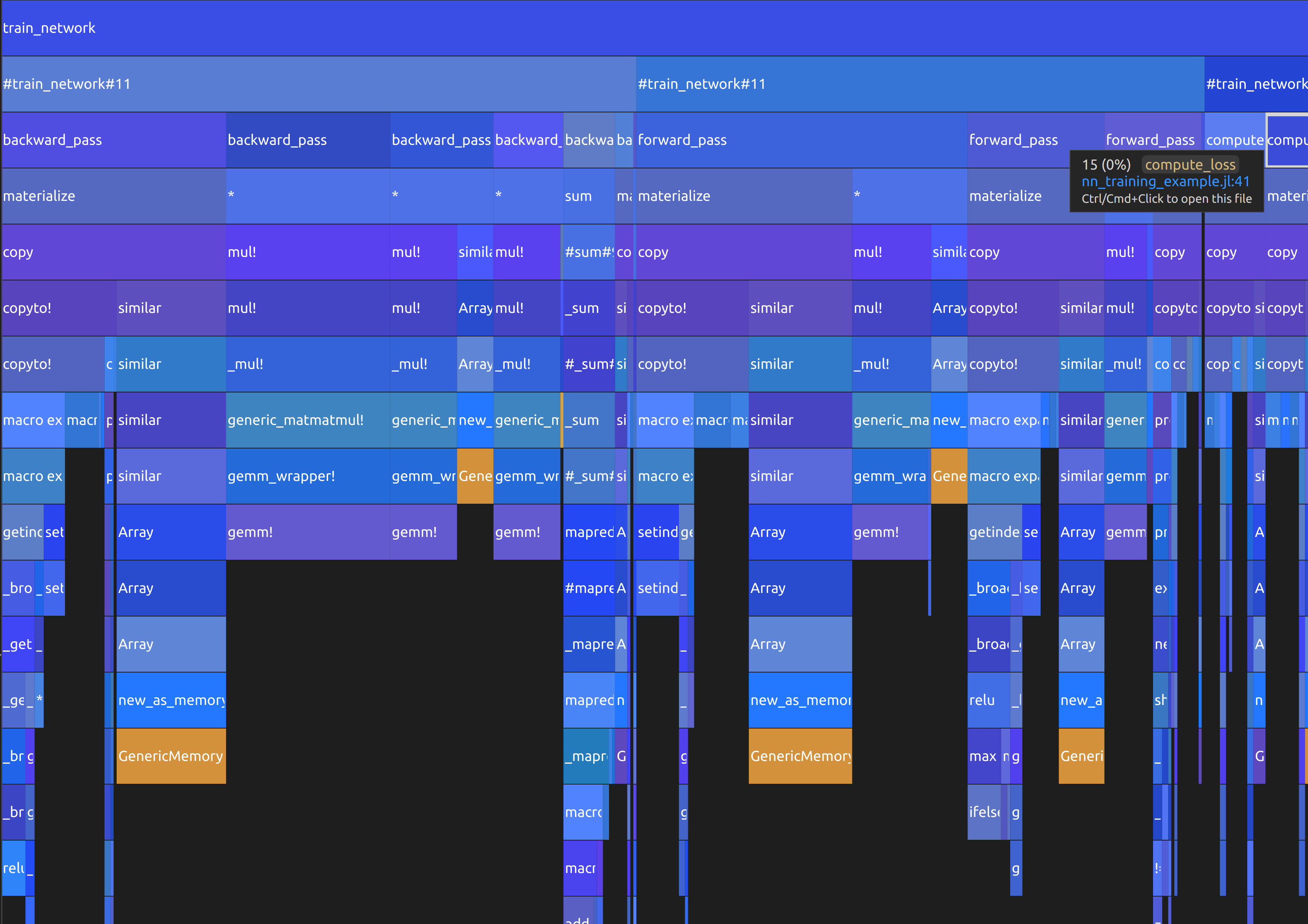
In the flame graph, you can see that most of the time is spent inside the backward_pass function, with forward_pass following closely behind. After this, compute_loss takes up some time, but update_parameters is not even visible. Additionally, the initialisation of the training loop is also dwarfed by the for loop. This type of graph can very quickly tell you which parts of your program to focus your attention on optimising. In this example, it only really makes sense to spend any effort on backward_pass, forward_pass and potentially compute_loss, as optimising anything else will not significantly speed up your training.

Summary

The statistical profiler is particularly useful for identifying:

• Functions that consume the most CPU time
• Unexpected bottlenecks in your code
• The call patterns that lead to slow execution
• Whether optimizations are having the intended effect

When using the statistical profiler, keep in mind:

• Run your code long enough to get meaningful samples (typically at least a few seconds)
• Run your function at least once so that you aren’t timing the JIT compilation
• The profiler adds some overhead, so don’t use it for final performance measurements
• Results may vary between runs due to the statistical nature of sampling
• Focus on the functions that consistently show up as hot spots across multiple profiling runs
• Reduce the input size to optimise on smaller examples first to increase development speed