Speed of Operations

This section is based off information from ithare.com, whose article is very well written and should be viewed.

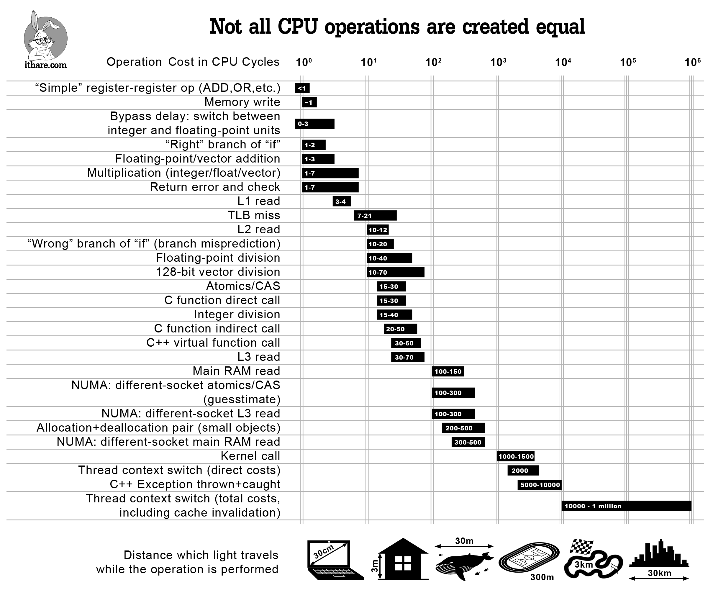
Taking a look at Figure 1, we can see that the basic operations, such as addition, multiplication and even memory writes are very fast, costing on the order of a single CPU cycle. The more interesting comparison is between cache reads and allocation. An L1 read costs a handful of cycles, while allocating and freeing even a small object costs a few hundred — orders of magnitude more than a simple numeric calculation. Note also the cost of a mispredicted branch: taking the “wrong” branch of an if costs roughly an order of magnitude more than taking the predicted one.

Modern CPUs use branch prediction to start executing one of the branches of an if statement before the condition has finished being evaluated. If the CPU gets the prediction wrong, then it has to backtrack which costs many cycles. This is one of the reasons you see many people opting for “branchless” programming styles, where control loops are kept to a minimum. This usually involves using boolean numerics to set a value to zero if something is false and one otherwise and then summing both results together. Branchless programming can have significant performance improvements if done correctly.

Let’s look at an example of branchless programming:

function branched_absolute(x)
    if x < 0
        return -x
    else
        return x
    end
end

function branchless_absolute(x)
    # Convert boolean to 0 or 1, then use arithmetic
    mask = x < 0
    return x * (1 - 2 * mask)
end

# Test with some data
x = rand(-100:100, 1000);

# Reduce with `sum` rather than `map`, so that we are not measuring the
# allocation of an output array instead of the branch itself.

import BenchmarkTools: @benchmark, @btime, @belapsed
display(@benchmark sum(branched_absolute, $x))

BenchmarkTools.Trial: 10000 samples with 772 evaluations per sample.
 Range (min … max):  164.417 ns … 394.119 ns  ┊ GC (min … max): 0.00% … 0.00%
 Time  (median):     168.938 ns               ┊ GC (median):    0.00%
 Time  (mean ± σ):   170.606 ns ±   7.983 ns  ┊ GC (mean ± σ):  0.00% ± 0.00%

     █▅ ▅█▂                                                      
  ▂▅▆██████▄▆▄▄▃▄▄▄▄▃▄▄▃▂▂▂▂▂▂▂▂▂▂▂▂▂▂▂▂▂▂▂▂▂▂▂▂▂▂▂▂▁▂▂▂▂▂▂▂▁▂▂ ▃
  164 ns           Histogram: frequency by time          205 ns <

 Memory estimate: 0 bytes, allocs estimate: 0.

display(@benchmark sum(branchless_absolute, $x))

BenchmarkTools.Trial: 10000 samples with 192 evaluations per sample.
 Range (min … max):  510.000 ns …  1.984 μs  ┊ GC (min … max): 0.00% … 0.00%
 Time  (median):     520.156 ns              ┊ GC (median):    0.00%
 Time  (mean ± σ):   532.423 ns ± 48.438 ns  ┊ GC (mean ± σ):  0.00% ± 0.00%

  ▆██▇▇▄▂▂▃▃▅▄▄▂▁                                              ▂
  ██████████████████▇▇▆▇█▇▆▆▆▆▆▄▄▅▄▆▄▆▄▅▁▅▅▆▅▄▄▅▃▅▃▅▄▄▅▃▄▅▄▁▅▃ █
  510 ns        Histogram: log(frequency) by time       745 ns <

 Memory estimate: 0 bytes, allocs estimate: 0.

The result is worth dwelling on, because it is the opposite of what the branchless story would predict: the hand-written branchless version is several times slower than the one with the if in it. The reason is that there was never a branch to remove in the first place. If you inspect the generated code with @code_llvm, branched_absolute compiles down to a single absolute-value instruction — the compiler recognised the pattern and emitted branchless code for you. Our “branchless” version, by contrast, compiles to a shift, an and, a subtract and an integer multiply, and integer multiplication is one of the slower arithmetic operations on the chart above. Both loops are vectorised, so we end up paying for four extra vector operations per batch of elements in exchange for removing a branch that had already been removed.

This is the general lesson. Branchless programming is a real technique, and it can pay off for genuinely unpredictable branches in a hot loop, but modern compilers already remove the easy cases. Rewriting readable code into arithmetic on booleans is a pessimisation far more often than it is an optimisation, and the only way to know which you have is to benchmark it.