Memory Usage

Hunting down allocations

All resources on a computer are usually finite. The resource which is usually considered first is time. How long will it take to run a certain piece of code? An equally important question is “how much memory will this algorithm use?“. Memory is also a finite resource and a developer should be considerate of the memory footprint his code has. Similar tools to what we have already discussed can be repurposed to measure how much memory has been used.

In the earlier section on software stack and heap, we spoke about the stack and the heap. Here, it is important to distinguish between them during profiling. The stack tends to be a lot smaller than the heap, and one should avoid allocating large objects on the stack. Often this can lead to crashes or poor performance. In the profiling techniques we have discussed, you will have seen that these techniques also measure the number of allocations, which refers to allocations on the heap. Additionally, most of the timing includes an estimate of the GC¹ time spent trying to the clean-up the memory allocated by the function.

Let’s take a look at profiling the function given, using the BenchmarkTools.jl package:

import BenchmarkTools: @benchmark, @btime
function mem_func(n, pow)
    arr = rand(n)
    s = 0
    for x in arr
        s += x ^ pow
    end
end
n = 1024;
pow = 3;
display(@btime mem_func($n, $pow));

1.480 μs (3 allocations: 8.08 KiB)
nothing

Notice that we are interpolating the variables n and pow by using the $ character. This should always be done to accurately benchmark a function with input arguments which come from variables. Secondly, notice that the output of this benchmark specifies that there was one allocation with a total of 8.12 KiB (which is 1024×8 = 8192 bytes). However, it does not tell us where the allocation is. For our function, it is easy to see that creating the array caused the allocation, however, in some code addressing where this comes from can be a challenge.

Julia v1.8 introduced an allocation profiler which allows you to profile your code and visually inspect where allocations are coming from. This new functionality is covered and demonstrated in a great talk from JuliaCon 2022 called “Hunting down allocations with Julia 1.8’s Allocation Profiler”². I will use the same example given to demonstrate how this works in practice. Take the example of serialising a CSV³ file with some data:

module TestAllocs
function serialise(rows::Vector{Vector{T}}) where {T}
    output = ""
    for row in rows
        for col_idx in eachindex(row)
            val = row[col_idx]
            output = output * string(val) # string concat
            if col_idx < length(row)
                output = output * ","
            end
        end
        # add a newline
        output = output * "\n"
    end
    return output
end
end

We can benchmark this code with some data:

rows = [rand(10) for _ in 1:128];
display(@benchmark TestAllocs.serialise($rows);)

BenchmarkTools.Trial: 2289 samples with 1 evaluation per sample.
 Range (min … max):  1.246 ms … 12.217 ms  ┊ GC (min … max): 14.18% … 17.84%
 Time  (median):     1.791 ms              ┊ GC (median):    21.47%
 Time  (mean ± σ):   2.177 ms ±  1.178 ms  ┊ GC (mean ± σ):  21.14% ±  4.94%

  ▃▇█▇▇▆▆▅▅▄▄▃▃▃▂▂▂▁   ▁      ▁                              ▁
  ████████████████████▇██▇▇▇▅▇█▇▆▆▄▅▆▆▅▁▅▆▆▅▇▆▄▅▅▆▅▅▅▅▄▅▅▅▆▅ █
  1.25 ms      Histogram: log(frequency) by time     7.45 ms <

 Memory estimate: 30.88 MiB, allocs estimate: 6400.

We can see that after compilation, we still have a huge amount of allocations present (over 5000 allocations), and a huge amount of time is spent garbage collecting. Instead of manually trying to figure out which lines are allocating, we can instead use a profiler to find this information out automatically. In order to do this, we must use the Profile.jl package, which is included in the base library. You can run

using Pkg; Pkg.add("Profile")

to add this to your environment. Now we can run the profiler, to specifically track the allocations⁴:

using Profile
Profile.Allocs.@profile sample_rate=1 TestAllocs.serialise(rows);

One can choose a sample rate between 0 and 1. It is recommended to use @time first to figure out how many allocations there are, and if there are many, to use a small sample rate. If you choose a number that is too large, this profile will take a very long time to finish. In order to visualise these allocations we will also use a package called PProf.jl (created by Google, which you will also need to install). You can run the following code to visualise the allocations in a web browser:

using PProf
PProf.Allocs.pprof(from_c=false)

The from_c parameter will allow you to filter out any stack frames internally allocated by the Julia runtime, which usually just clutters up your results. You will get a link to a localhost website (locally hosted on your machine), which lets you view the results.

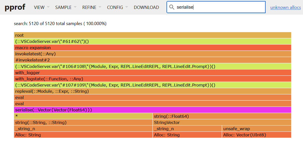
If you change the view to a flame graph (View->Flame Graph) you can see something like the figure above. Changing the sample from allocs to size (Sample->size) will weight the size of each block by the size. The bars at the bottom are the most useful as these refer to the lowest level calls. You can see that the problem function is our serialise function. Use the search bar to highlight this function call. Once highlighted, you can switch to the source view, which will highlight for us where all the allocations come from.

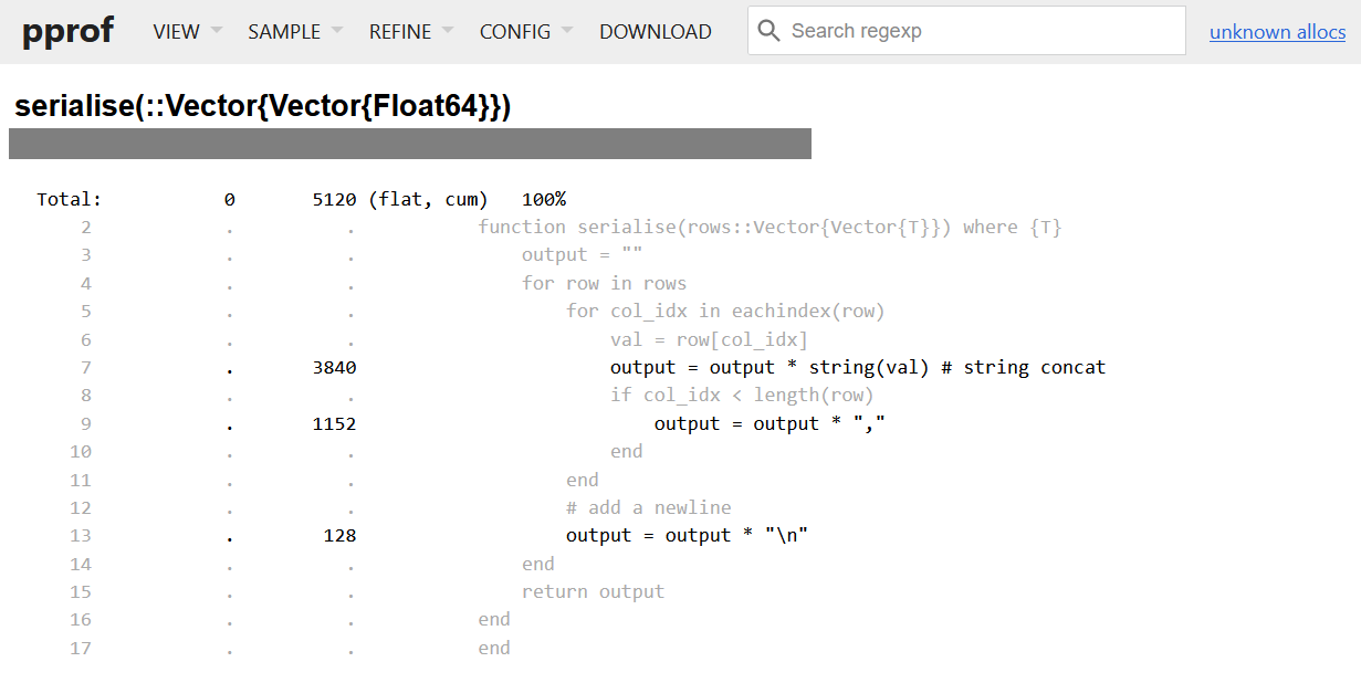
Looking at the source view, we can see that we are allocating a lot whenever we are concatenating a string, and also when converting a value to a string. Each concatenation produces a new string which causes another allocation. Instead of concatenating, we want to print to a buffer instead. Let’s look at an improved version of this code:

module TestAllocsFast
function serialise(rows::Vector{Vector{T}}) where {T}
    buffer = IOBuffer()
    for row in rows
        for col_idx in eachindex(row)
            val = row[col_idx]
            print(buffer, val)
            if col_idx < length(row)
                print(buffer, ",")
            end
        end
        # add a newline
        print(buffer, "\n")
    end
    return String(take!(buffer))
end
end

If we rerun the results, we can see a huge performance improvement:

display(@benchmark TestAllocsFast.serialise($rows))

BenchmarkTools.Trial: 10000 samples with 1 evaluation per sample.
 Range (min … max):  63.400 μs … 979.500 μs  ┊ GC (min … max):  0.00% … 90.78%
 Time  (median):     69.200 μs               ┊ GC (median):     0.00%
 Time  (mean ± σ):   87.084 μs ±  68.517 μs  ┊ GC (mean ± σ):  12.50% ± 14.26%

  █▇▆▄▂▁                                                       ▂
  ████████▇█▇▆▇██▇▆▆▇▇▇▆▆▇▇▆▆▆▆▅▅▅▄▅▅▅▆▁▅▅▄▅▅▆▆▆▇▆▇▇▇▇▇▇▆▇▆▆▆▆ █
  63.4 μs       Histogram: log(frequency) by time       397 μs <

 Memory estimate: 591.39 KiB, allocs estimate: 3858.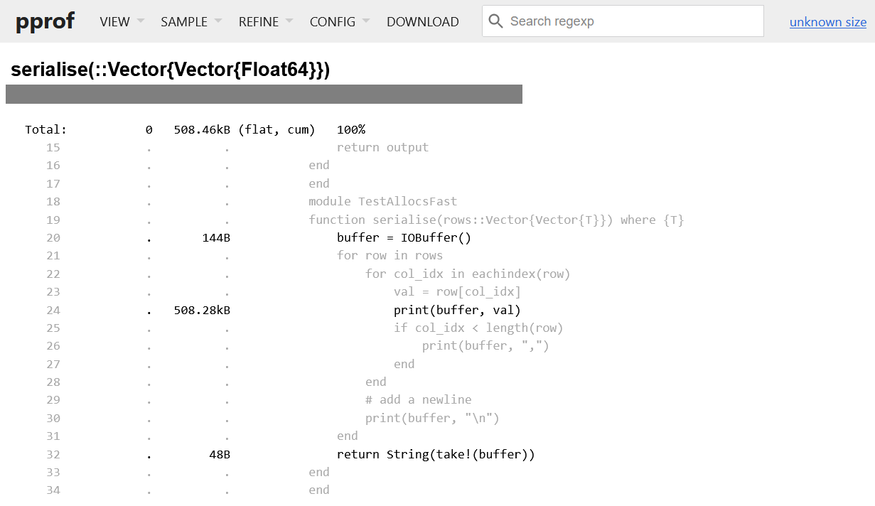

We can see from the faster version that the allocations are much improved in terms of size, but there are still lines which allocate. This implementation is not completely optimised, but it has improved hugely on the previous implementation. The advantage of this profiling approach is that you can find allocations that you may not have realised are there.

Conclusion

While these practical methods give you a wide array of tools, which can be used to analyse runtime metrics, they do not give you the full picture about the performance of the studied algorithms. For one, each of the performance metrics are specific to the hardware on which the benchmarks were run. This makes it almost impossible for different researchers to compare their results via these empirical methods, unless they are running each algorithm on the same hardware. Alongside empirical benchmarks, we must also have a set of theoretical tools which can be used to quantify the performance of an algorithm. This is going to be the topic of the next section.