CUDA Kernels

When writing code for the GPU, the best practice is to first try and use array programming, which can be executed on either the CPU or the GPU. This code is easy to test, and the tests can be run on any machine, without the GPU. If the code works correctly on the CPU, it is highly likely to also work on the GPU - as long as there are no errors. However, there will always be edge cases when your algorithm cannot be implemented in terms of array and broadcast operations, or it is highly inefficient to do so. In these cases, you may have to write the GPU kernel itself.

A GPU kernel is a self-contained program that can be run independently across many cores of a GPU. Traditionally, GPUs could compile shaders, which were able to calculate the colour of a single pixel on the screen. This shader would be run for every pixel to colour a final image. Kernels are just like these old shaders, but perform generic computation, instead of a graphics processing routine. Instead of iterating over each unit of work, we simply describe how to do a single piece of the work, given some identification of what work one should be doing.

Let’s take the example of writing a basic shader which performs vector addition. Luckily, even though CUDA is designed to be a C-like language, we are able to write all of our CUDA code in native Julia (with the help of CUDA.jl for compilation). As a starting point, let’s write a basic for loop that would be executed on the GPU:

function basic_vec_add!(c, a, b)
    for i in eachindex(c, a, b)
        @inbounds c[i] = a[i] + b[i]
    end
    return nothing
end

This code will add the vectors a and b together and store the result in the vector c. Our CUDA kernel should make each core perform one of these inner loop additions. We are able to specify which core should do the work through the use of some special variables which are provided to each core when the kernel is scheduled for execution. Take the following example:

function basic_vec_add_cuda!(c, a, b)
    i = threadIdx().x
    if i <= length(c)
        @inbounds c[i] = a[i] + b[i]
    end
    return nothing
end

Here, we have used the threadIdx function which gives us a named tuple with x, y and z components. This is an identifier to the core as to which thread of work it is assigned. CUDA uses a thread based model for execution; each thread executes the code in the kernel independently of one another.

We can compile and launch this kernel on the GPU with the following syntax:

a = CUDA.rand(128); b = CUDA.rand(128); c = similar(a);
@cuda threads=length(c) basic_vec_add_cuda!(c, a, b);
isapprox(c, a.+b)

We can see that our kernel worked as expected, despite the use of scalar indexing. The @cuda macro compiles and launches the function specified. We additionally have to specify the number of threads used as the length of the vector input. The CUDA programming model uses a geometric partitioning system. The system can be explained as:

• Each GPU has a 3-dimensional grid of blocks.
• Each block contains a 3-dimensional group of threads.
• Each thread is executed independently.

In our case, we restricted the execution to a single dimension $x$x, but this just makes the number of elements in the $y$y and $z$z dimensions equal to $1$1. One important restriction in the CUDA programming model is making sure that a block has a maximum number of possible threads. This limit is usually $1024$1024 threads. As we are often dealing with larger arrays, we need to make use of multiple blocks to allow execution across more threads than this limit.

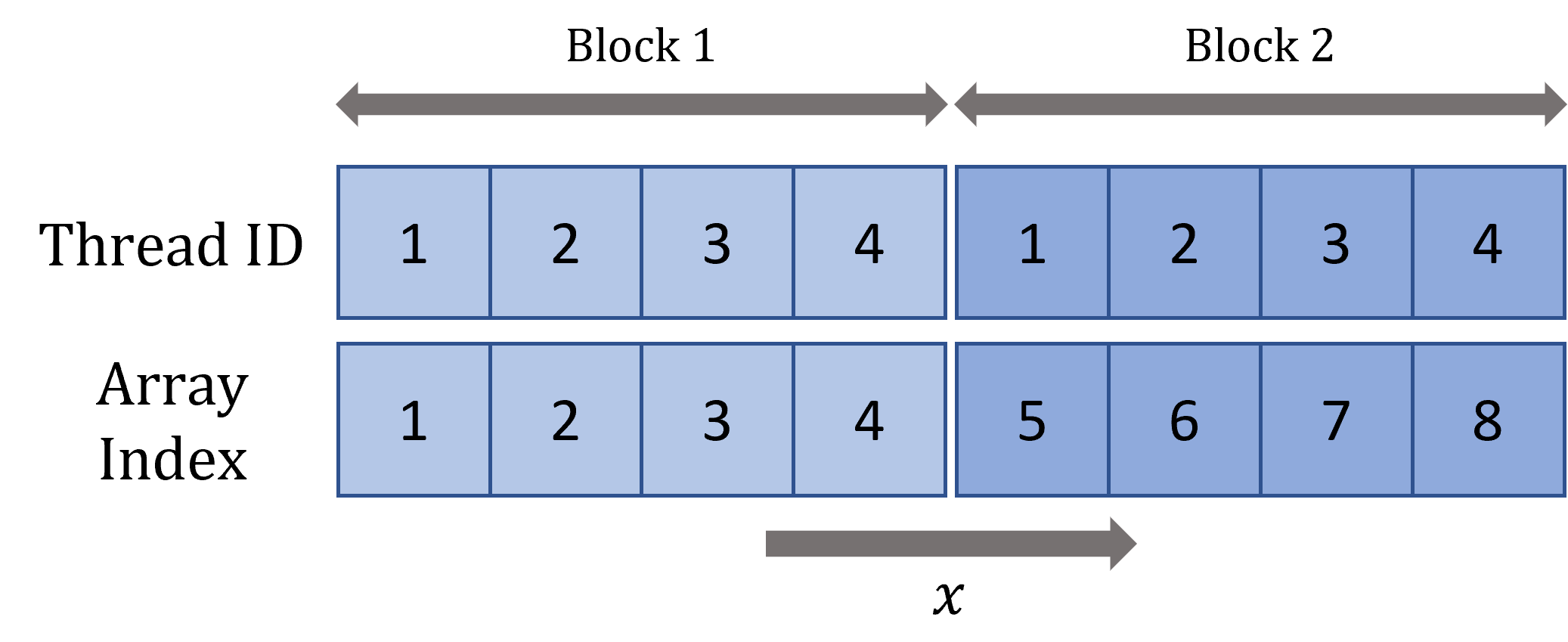
Looking at the figure above, we can visualise how the indexing scheme works in a single dimension. Each block has $4$4 assigned threads whose indices begin at $1$1 and end at $4$4. Each block also has an index which goes from $1$1 to $2$2. This is enough to map to each element in the example $8$8 element array. We can adjust our kernel to take into account block sizes:

function basic_vec_add_cuda!(c, a, b)
    i = (blockIdx().x - 1) * blockDim().x + threadIdx().x
    if i <= length(c)
        @inbounds c[i] = a[i] + b[i]
    end
    return nothing
end

Now, we write a wrapper around the add function which works on CUDA arrays, which will automatically calculate the number of blocks and threads needed.

function basic_vec_add!(c::CuArray, a::CuArray, b::CuArray)
    n = length(c)
    @assert n == length(a) == length(b)

    num_threads = min(1024, n)
    num_blocks = cld(n, 1024)
    @cuda blocks=num_blocks threads=num_threads basic_vec_add_cuda!(c, a, b)

    return nothing
end

Notice that for an input of length $1029$1029, a total of $2048$2048 threads will be launched. It is now up to you as the programmer to decide how many threads to launch.

A common pattern seen throughout custom kernel launches is to grab the number of threads from a configuration provided by CUDA for a compiled kernel. This is then used to assign blocks.

function basic_vec_add!(c::CuArray, a::CuArray, b::CuArray)
    n = length(c)
    if n == 0
        return nothing
    end

    @assert n == length(a) == length(b)

    kernel = @cuda name="basic_vec_add" launch=false basic_vec_add_cuda!(c, a, b)
    config = launch_configuration(kernel.fun)
    threads = min(n, config.threads)
    blocks = cld(n, threads)
    kernel(c, a, b; threads=threads, blocks=blocks)

    return nothing
end

One should note that CUDA also has maximum sizes for blocks and grids. However, when getting to the grid level, one is very unlikely to have an array large enough to cause an issue. For example, the maximum dimensions on this graphics card are:

@show CUDA.max_block_size
@show CUDA.max_grid_size

CUDA.max_block_size = (x = 1024, y = 1024, z = 64)
CUDA.max_grid_size = (x = 2147483647, y = 65535, z = 65535)

The maximum size of a block is the product of the dimensions:

@show reduce(*, CUDA.max_block_size)

reduce(*, CUDA.max_block_size) = 67108864

As long as the dimensions you choose to multiply to a number less than the above, you do not need to use the grid.

Now there are some things that you may have noticed that seemed to reduce performance. For example, we are including an if statement in our kernel. This is necessary as the length of the array may not be easily split up into blocks. We are manually performing our bound checking here to ensure that we can safely read and write from memory. This is true in the case of an array of length $1029$1029, which would have $1023$1023 threads running which would index outside the array. To ensure this does not happen, we must guard with the manual bounds checking.

Additionally, CUDA imposes on us the restriction of returning nothing from the kernels. All memory allocations must be done outside the kernel. This usually means implementing your kernel as an in-place operation on pre-allocated memory. If you want to provide a better API for users and abstract away the allocations, one can wrap the call to the kernel:

function basic_vec_add(a::CuArray, b::CuArray)
    c = similar(a)
    basic_vec_add!(c, a, b)
    return c
end

Additionally, if the memory is only needed temporarily, you can create it outside the function and release it later. If you are writing the critical loop section of your code, it is often better to write the main algorithm with pre-allocated caches and then create a wrapper (like the one above) to optionally use if you do not want the users of the code to manually manage their cache. This gives the option for re-using a cache in a hot-loop.